šŸ‘ļø … visits

Simulations in motion

Movies

Explore shear-driven turbulence, magnetic-field stretching, and supernova remnants. Choose a movie below or rotate a remnant in three dimensions.

Kelvin–Helmholtz instability

Start with the two three-dimensional tours, then explore the evolving density, magnetic-field stretching, and vorticity. Use full screen to inspect fine structures and panel labels.

Density fly-through

0:28 Ā· 15 MB

Travel through the density structure of a Kelvin–Helmholtz simulation.

Scientific details

A flight through the density field at a fixed time, $t/t_\Delta \simeq 200$, in a Mach 1 Kelvin–Helmholtz simulation with $\mathrm{Re}_\Delta = 16384$ and $\mathrm{Pm}_\Delta = 1$. Color shows the logarithmic density contrast, $\ln(\rho/\rho_0)$.

Download MP4

Magnetic-field fly-through

0:28 Ā· 42 MB

Follow the magnetic-field geometry through the same density snapshot.

Scientific details

Magnetic-field lines shown as white tubes over the density field at $t/t_\Delta \simeq 200$, with Mach 1, $\mathrm{Re}_\Delta = 16384$, and $\mathrm{Pm}_\Delta = 1$. Color shows $\ln(\rho/\rho_0)$.

Download MP4

Density and magnetic-field stretching

0:15 Ā· 30 MB

Compare density and field-aligned stretching in two perpendicular planes.

Scientific details

Density and magnetic-field stretching in the $xy$ and $yz$ planes of the Mach 1 simulation. The density panels show $\rho/\langle\rho\rangle_0$, while the adjacent panels show the dimensionless stretching rate, $t_\Delta \hat{B}_i\hat{B}_j\partial_j u_i$. The Reynolds number is $\mathrm{Re}_\Delta = 16384$ and the magnetic Prandtl number is $\mathrm{Pm}_\Delta = 1$.

Download MP4

Vorticity in the xy plane

0:21 Ā· 31 MB

Compare ten Reynolds numbers in a slice through the shear layers.

Scientific details

Vorticity magnitude in the $xy$ plane near $z/L = 0$. The ten panels compare Reynolds numbers from $\mathrm{Re}_\Delta = 64$ to $16,\!384$ at Mach 1 and $\mathrm{Pm}_\Delta = 1$. Color shows $t_\Delta |\nabla\times\boldsymbol{u}|$.

The sequence extends to $t/t_\Delta=1,\!000$. The $\mathrm{Re}_\Delta=64$ and $4,\!096$ panels hold their final saved states at $t/t_\Delta=700$ and $943.1$, respectively; the other eight runs reach $1,\!000$.

Download MP4

Vorticity in the yz plane

0:21 Ā· 32 MB

View the same Reynolds-number sequence from a perpendicular direction.

Scientific details

Vorticity magnitude in the $yz$ plane near $x/L = -1/4$. The ten panels compare $\mathrm{Re}_\Delta = 64$ to $16,\!384$ at Mach 1 and $\mathrm{Pm}_\Delta = 1$. Color shows $t_\Delta |\nabla\times\boldsymbol{u}|$.

The sequence extends to $t/t_\Delta=1,\!000$. The $\mathrm{Re}_\Delta=64$ and $4,\!096$ panels hold their final saved states at $t/t_\Delta=700$ and $943.1$, respectively; the other eight runs reach $1,\!000$.

Download MP4

Supernova remnants

Cooling remnants extracted from galactic disk simulations in Beattie et al. (2025).

Supernova remnants as turbulence engines

0:26 Ā· 18 MB

Compare baroclinic sources in blue with vorticity in red.

Scientific details

An animated version of Figure 2 from Beattie (2025), submitted to ApJL, where I derive the power spectrum relation between a baroclinic source and an incompressible turbulence spectrum, which has direct applications for supernova-driven turbulence. Each panel is a supernova remnant, and the slider shows between the baroclinic magnitude (blue) and the vorticity magnitude (red).

Download MP4

Explore supernova remnants in 3D

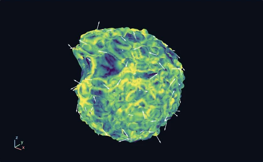
Choose a remnant, compare its fields and vector overlays, and explore their probability density functions.

Interactive scientific explorer

SNR 26 Output 00030

Compare remnant structure, vector fields, and the distributions beneath them.

Each remnant loads on demand. Output labels identify snapshots, not a time sequence of the same remnant.

SNR 26: vorticity magnitude with vorticity arrows

SNR 26 Ā· vorticity magnitude and arrows

The preset loads about 5–7 MB. Drag to rotate Ā· scroll or pinch to zoom.

Ready to explore. The simulation data load when you open the viewer.

Explore the fields

The preset loads a fixed diagnostic shell. Full-volume mode loads about 13–21 MB per field group as needed.

Arrows show the full three-dimensional direction at the shell.

Coordinates follow x, y, z. The cutaway removes the higher-coordinate side of the shell and arrows.

What the surface and arrows represent

The original preset follows the 95th percentile of the baroclinic-source magnitude, smoothed over 0.8 voxels. Full-volume mode extracts a new isosurface at the chosen field value across the whole 128³ cutout, including material outside the remnant mask. The level is divided by the field’s interior mean or RMS. Smoothing changes only the shape field. Geometry stays fixed when the color field changes. These diagnostic isosurfaces are not fitted shock fronts. Classical marching cubes can resolve ambiguous cells differently from the original preset.

Density, pressure, and the temperature proxy P/ρ are divided by their mean within the remnant mask. Vorticity and baroclinic-source magnitudes are divided by their RMS within that mask. These positive fields use logarithmic colors, limited to their surface 2nd–98th percentiles. Values outside the scale saturate at the end colors. Physical-unit conversions are not assumed.

Here b = āˆ‡Ļ Ɨ āˆ‡P / ρ² is the physical baroclinic source. The signed quantity ω Ā· b shows the baroclinic contribution to the evolution of |ω|²/2. Positive values reinforce existing vorticity, while negative values oppose it. It is one contribution to the enstrophy budget. The alignment view separates direction from magnitude.

Arrows sample the selected vector at well-spaced locations on the current surface. Full-volume mode uses farthest-point sampling from up to 4,000 candidate vertices. Equal-length arrows show direction. With magnitude scaling enabled, lengths are proportional to magnitude up to the 95th percentile of up to 800 sampled vectors. Velocity is shown in the simulation frame, without subtracting remnant motion. Vorticity arrows mark rotation axes, not flow trajectories. Increasing transparency reveals arrows behind the surface but blends the surface colors.

PDFs span the full finite range of the selected quantity, including values beyond the color limits. Surface PDFs update with the geometry and approximate area weighting by assigning one third of each triangle’s area to each vertex. Interior PDFs use equal-volume cells in the remnant mask. Each PDF integrates to one over its included samples. Logarithmic quantities have a density per unit log₁₀. Vector PDFs use the magnitude of the interpolated vector and its interior RMS. Cutaways, camera views, and arrow counts do not filter these distributions.

Full-volume data retain the original float32 values with lossless compression. Temperature is reconstructed as P/ρ and magnitudes from the saved vector components. Colors and vectors use trilinear interpolation on the original grid. Fast geometry samples the smoothed shape field on a 64³ grid spanning the same cutout. Surface PDFs describe that displayed mesh. The slice is sampled at 128² points, and its contour lines use linear interpolation within triangles. Undefined color values appear gray.

View field definitions and export metadata